import numpy as np
import scipy.stats as st

from matplotlib import pyplot as plt
from matplotlib.ticker import AutoMinorLocator
import seaborn as sns

import warnings
warnings.filterwarnings('ignore')Statistics classes in social sciences, during an undergraduate degree, revolve around p-values mainly. Despite that, I have never seen the mention of p-value distributions. So, here we go:
How does the p-value distribution look like when there is no effect?
p_val_list = [] # a bag to hold p-values

for i in range(0, 1000000):
    ctrl = np.random.normal(loc=100, scale=15, size=51) # sampling from a normal distribution with mean 100, std 15
    trt = np.random.normal(loc=100, scale=15, size=51) # sampling from a normal distribution with mean 100, std 15
    p_val = st.ttest_ind(trt, ctrl)[1]  # doing a t-test and grabbing the p-value

    p_val_list.append(p_val) # storing the p-value in the bag
fig = plt.figure(figsize=(9, 5))
ax = fig.add_subplot(1, 1, 1)
plt.ticklabel_format(style='plain', axis='y')
ax.hist(p_val_list, bins=100, edgecolor='black', linewidth=.9)
ax.xaxis.set_minor_locator(AutoMinorLocator(5))
ax.yaxis.set_minor_locator(AutoMinorLocator(5))
ax.tick_params(which='both', width=2)
ax.tick_params(which='major', length=7)
ax.tick_params(which='minor', length=4)
ax.set_ylim(0, 1000000)
plt.title('When the true effect size = 0')Text(0.5, 1.0, 'When the true effect size = 0')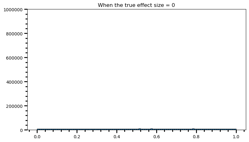
Every p-value is equally likely. That’s why chosen alpha level corresponds to how often you will fool yourself in the long run, when there is no effect.
If the chosen alpha level is .10, then under the null hypothesis 10 percent of the p-values fall below 0.10.
power = [val for val in p_val_list if val <= 0.05] # .05 is the chosen for alpha
print('Power: ', round(len(power) / len(p_val_list), 2))
Power: 0.05This is our long-term type I error rate, since theoretically the power is undefined in this case (i.e., the null is the truth). We don’t expect to fool ourselves more than 5% in the long run, when there is no effect.
Let’s see what happens when there is an effect:
p_val_list = []

for i in range(0, 1000000):
    ctrl = np.random.normal(loc=100, scale=15, size=51)
    trt = np.random.normal(loc=104.5, scale=15, size=51)
    p_val = st.ttest_ind(trt, ctrl)[1]

    p_val_list.append(p_val)
fig = plt.figure(figsize=(9, 5))
ax = fig.add_subplot(1, 1, 1)
plt.ticklabel_format(style='plain', axis='y')
ax.hist(p_val_list, bins=100, edgecolor='black', linewidth=.9)
ax.axhline(y=10000, color='r', linestyle='--')
ax.xaxis.set_minor_locator(AutoMinorLocator(5))
ax.yaxis.set_minor_locator(AutoMinorLocator(5))
ax.tick_params(which='both', width=2)
ax.tick_params(which='major', length=7)
ax.tick_params(which='minor', length=4)
ax.set_ylim(0, 1000000)
plt.title('For Cohen\'s d of 0.3')Text(0.5, 1.0, "For Cohen's d of 0.3")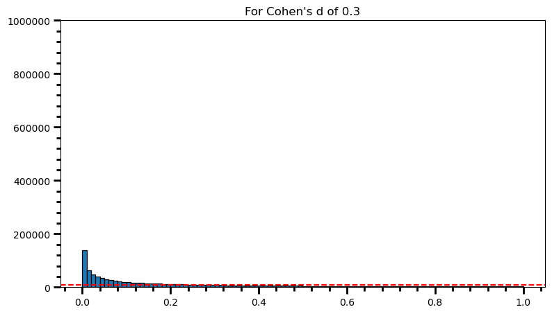
power = [val for val in p_val_list if val <= 0.05] # .05 is the chosen for alpha
print('Power: ', round(len(power) / len(p_val_list), 2))
Power: 0.32fig = plt.figure(figsize=(9, 5))
ax = fig.add_subplot(1, 1, 1)
plt.ticklabel_format(style='plain', axis='y')
ax.hist([val for val in p_val_list if val <= .05], bins=5, edgecolor='black', linewidth=.9)
ax.axhline(y=10000, color='r', linestyle='--')
# ax.xaxis.set_minor_locator(AutoMinorLocator(5))
ax.yaxis.set_minor_locator(AutoMinorLocator(5))
ax.tick_params(which='both', width=2)
ax.tick_params(which='major', length=7)
ax.tick_params(which='minor', length=4)
ax.set_xlim(0, 0.05)
ax.set_ylim(0, 1000000)
plt.title('For Cohen\'s d of 0.3')Text(0.5, 1.0, "For Cohen's d of 0.3")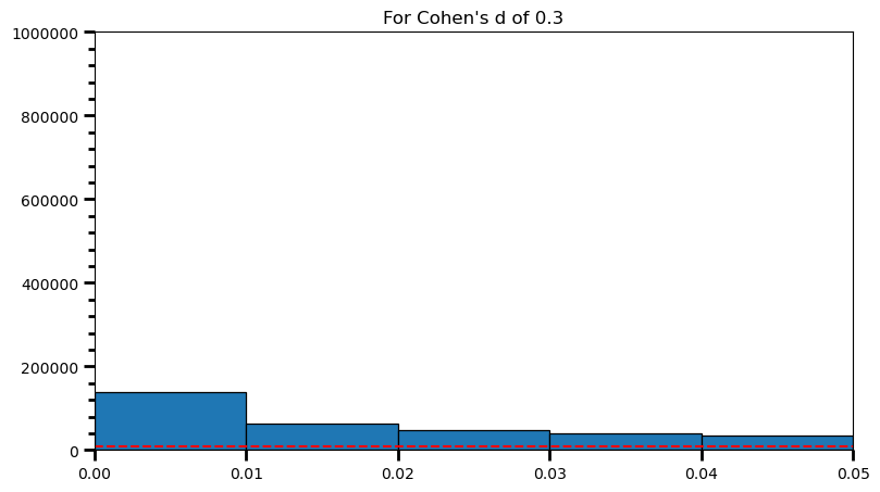
p_val_list = []

for i in range(0, 1000000):
    ctrl = np.random.normal(loc=100, scale=15, size=51)
    trt = np.random.normal(loc=107.5, scale=15, size=51)
    p_val = st.ttest_ind(trt, ctrl)[1]

    p_val_list.append(p_val)
fig = plt.figure(figsize=(9, 5))
ax = fig.add_subplot(1, 1, 1)
plt.ticklabel_format(style='plain', axis='y')
ax.hist(p_val_list, bins=100, edgecolor='black', linewidth=.9)
ax.axhline(y=10000, color='r', linestyle='--', alpha=.5)
ax.xaxis.set_minor_locator(AutoMinorLocator(5))
ax.yaxis.set_minor_locator(AutoMinorLocator(5))
ax.tick_params(which='both', width=2)
ax.tick_params(which='major', length=7)
ax.tick_params(which='minor', length=4)
ax.set_ylim(0, 1000000)
plt.title('For Cohen\'s d of 0.5')Text(0.5, 1.0, "For Cohen's d of 0.5")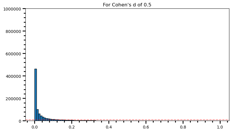
power = [val for val in p_val_list if val <= 0.05] # .05 is the chosen for alpha
print('Power: ', round(len(power) / len(p_val_list), 2))
Power: 0.71fig = plt.figure(figsize=(9, 5))
ax = fig.add_subplot(1, 1, 1)
plt.ticklabel_format(style='plain', axis='y')
ax.hist([val for val in p_val_list if val <= .05], bins=5, edgecolor='black', linewidth=.9)
ax.axhline(y=10000, color='r', linestyle='--')
# ax.xaxis.set_minor_locator(AutoMinorLocator(5))
ax.yaxis.set_minor_locator(AutoMinorLocator(5))
ax.tick_params(which='both', width=2)
ax.tick_params(which='major', length=7)
ax.tick_params(which='minor', length=4)
ax.set_xlim(0, 0.05)
ax.set_ylim(0, 1000000)
plt.title('For Cohen\'s d of 0.5')Text(0.5, 1.0, "For Cohen's d of 0.5")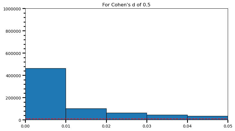
p_val_list = []

for i in range(0, 1000000):
    ctrl = np.random.normal(loc=100, scale=15, size=51)
    trt = np.random.normal(loc=109.5, scale=15, size=51)
    p_val = st.ttest_ind(trt, ctrl)[1]

    p_val_list.append(p_val)
fig = plt.figure(figsize=(9, 5))
ax = fig.add_subplot(1, 1, 1)
plt.ticklabel_format(style='plain', axis='y')
ax.hist(p_val_list, bins=100, edgecolor='black', linewidth=.9)
ax.axhline(y=10000, color='r', linestyle='--', alpha=.5)
ax.xaxis.set_minor_locator(AutoMinorLocator(5))
ax.yaxis.set_minor_locator(AutoMinorLocator(5))
ax.tick_params(which='both', width=2)
ax.tick_params(which='major', length=7)
ax.tick_params(which='minor', length=4)
ax.set_ylim(0, 1000000)
plt.title('For Cohen\'s d of 0.7')Text(0.5, 1.0, "For Cohen's d of 0.7")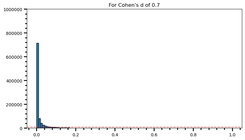
power = [val for val in p_val_list if val <= 0.05] # .05 is the chosen for alpha
print('Power: ', round(len(power) / len(p_val_list), 2))
Power: 0.89fig = plt.figure(figsize=(9, 5))
ax = fig.add_subplot(1, 1, 1)
plt.ticklabel_format(style='plain', axis='y')
ax.hist([val for val in p_val_list if val <= .05], bins=5, edgecolor='black', linewidth=.9)
ax.axhline(y=10000, color='r', linestyle='--')
# ax.xaxis.set_minor_locator(AutoMinorLocator(5))
ax.yaxis.set_minor_locator(AutoMinorLocator(5))
ax.tick_params(which='both', width=2)
ax.tick_params(which='major', length=7)
ax.tick_params(which='minor', length=4)
ax.set_xlim(0, 0.05)
ax.set_ylim(0, 1000000)
plt.title('For Cohen\'s d of 0.7')Text(0.5, 1.0, "For Cohen's d of 0.7")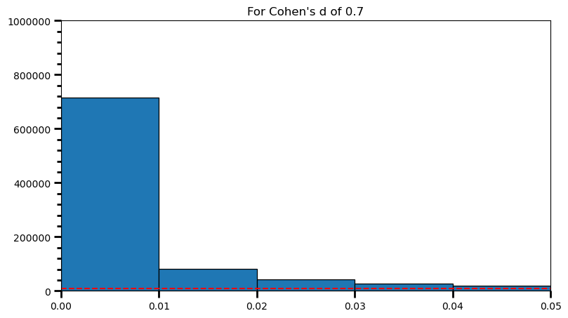
print(len([val for val in p_val_list if val >= .00 and val <= .01]) / len(p_val_list))0.715716p_val_list = []
for i in range(0, 1000000):
ctrl = np.random.normal(loc=100, scale=15, size=51)
trt = np.random.normal(loc=112, scale=15, size=51)
p_val = st.ttest_ind(trt, ctrl)[1]
p_val_list.append(p_val)fig = plt.figure(figsize=(9, 5))
ax = fig.add_subplot(1, 1, 1)
plt.ticklabel_format(style='plain', axis='y')
ax.hist(p_val_list, bins=100, edgecolor='black', linewidth=.9)
ax.axhline(y=10000, color='r', linestyle='--')
ax.xaxis.set_minor_locator(AutoMinorLocator(5))
ax.yaxis.set_minor_locator(AutoMinorLocator(5))
ax.tick_params(which='both', width=2)
ax.tick_params(which='major', length=7)
ax.tick_params(which='minor', length=4)
ax.set_xticks(np.arange(0, 1, 0.05))
ax.set_ylim(0, 1000000)
plt.title('For Cohen\'s d of 0.8')Text(0.5, 1.0, "For Cohen's d of 0.8")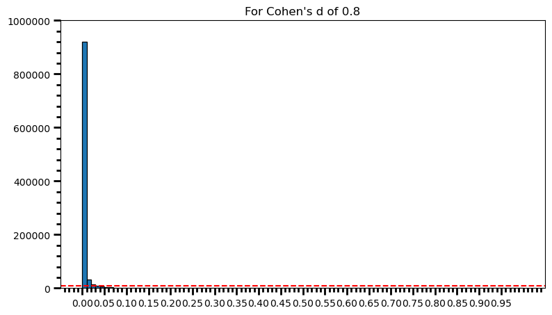
fig = plt.figure(figsize=(9, 5))
ax = fig.add_subplot(1, 1, 1)

plt.ticklabel_format(style='plain', axis='y')

ax.hist([val for val in p_val_list if val <= .05], bins=5, edgecolor='black', linewidth=.9)
ax.axhline(y=10000, color='r', linestyle='--')

# ax.xaxis.set_minor_locator(AutoMinorLocator(5))
ax.yaxis.set_minor_locator(AutoMinorLocator(5))
ax.tick_params(which='both', width=2)
ax.tick_params(which='major', length=7)
ax.tick_params(which='minor', length=4)

ax.set_xlim(0, 0.05)
ax.set_ylim(0, 1000000)
plt.title('For Cohen\'s d of 0.8')
Text(0.5, 1.0, "For Cohen's d of 0.8")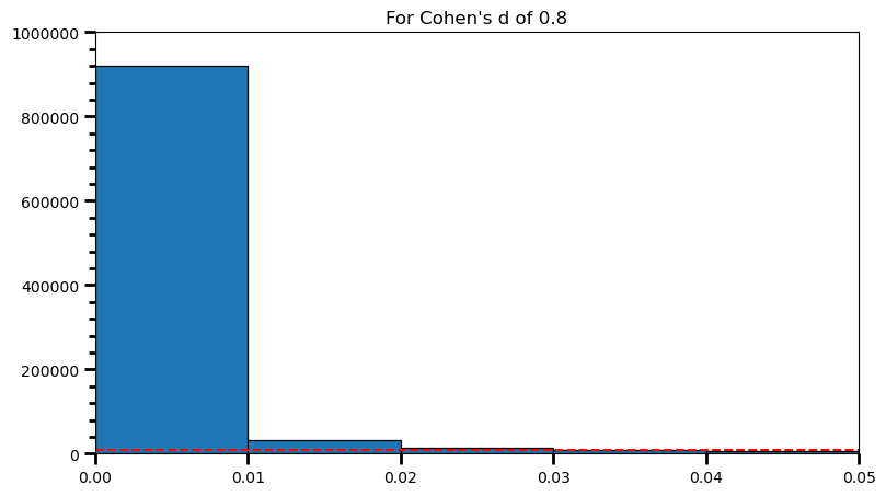
print(len([val for val in p_val_list if val >= .04 and val <= .05]) / len(p_val_list), '\n',
      len([val for val in p_val_list if val >= .03 and val <= .04]) / len(p_val_list), '\n',
      len([val for val in p_val_list if val >= .02 and val <= .03]) / len(p_val_list), '\n',
      len([val for val in p_val_list if val >= .01 and val <= .02]) / len(p_val_list), '\n',
      len([val for val in p_val_list if val >= .00 and val <= .01]) / len(p_val_list))
0.005389
0.008187
0.014401
0.032377
0.91928power = [val for val in p_val_list if val <= 0.05] # .05 is the chosen for alpha
print('Power: ', round(len(power) / len(p_val_list), 2))Power: 0.98As the statistical power increases, distribution of p-values pile up at the very left: Some p-values below 0.05 become more likely (ones more close to 0.00). And when you have very high power, certain p-values below 0.05 (relatively high ones) become more likely under the null:
Hence, wouldn’t be wise to reject the null despite p-value < .05
p_val_list = []

for i in range(0, 1000000):
    ctrl = np.random.normal(loc=100, scale=15, size=65) # different sample size
    trt = np.random.normal(loc=107.5, scale=15, size=65) # different sample size
    p_val = st.ttest_ind(trt, ctrl)[1]

    p_val_list.append(p_val)
power = [val for val in p_val_list if val <= 0.05] # .05 is the chosen for alpha
print('Power: ', round(len(power) / len(p_val_list), 2))Power: 0.81fig = plt.figure(figsize=(9, 5))
ax = fig.add_subplot(1, 1, 1)
plt.ticklabel_format(style='plain', axis='y')
ax.hist(p_val_list, bins=100, edgecolor='black', linewidth=.9)
ax.xaxis.set_minor_locator(AutoMinorLocator(5))
ax.yaxis.set_minor_locator(AutoMinorLocator(5))
ax.tick_params(which='both', width=2)
ax.tick_params(which='major', length=7)
ax.tick_params(which='minor', length=4)
ax.set_xticks(np.arange(0, 1, 0.05))
ax.set_ylim(0, 1000000)
plt.title('For Cohen\'s d of 0.5')Text(0.5, 1.0, "For Cohen's d of 0.5")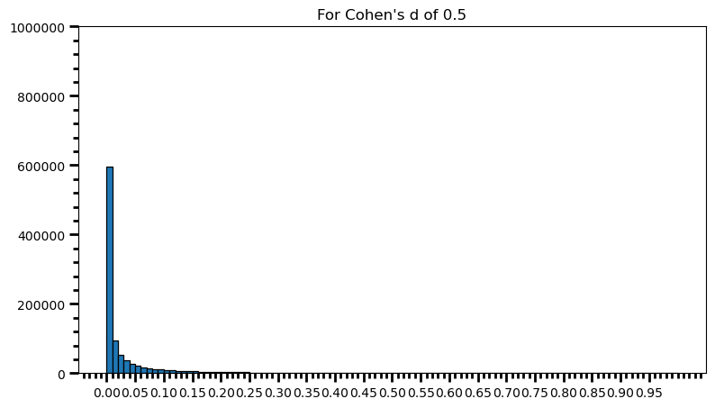
p_val_list = []

for i in range(0, 1000000):
    ctrl = np.random.normal(loc=100, scale=15, size=100) # different sample size
    trt = np.random.normal(loc=107.5, scale=15, size=100) # different sample size
    p_val = st.ttest_ind(trt, ctrl)[1]

    p_val_list.append(p_val)
power = [val for val in p_val_list if val <= 0.05] # .05 is the chosen for alpha
print('Power: ', round(len(power) / len(p_val_list), 2))Power: 0.94fig = plt.figure(figsize=(9, 5))
ax = fig.add_subplot(1, 1, 1)
plt.ticklabel_format(style='plain', axis='y')
ax.hist(p_val_list, bins=100, edgecolor='black', linewidth=.9)
ax.xaxis.set_minor_locator(AutoMinorLocator(5))
ax.yaxis.set_minor_locator(AutoMinorLocator(5))
ax.tick_params(which='both', width=2)
ax.tick_params(which='major', length=7)
ax.tick_params(which='minor', length=4)
ax.set_xticks(np.arange(0, 1, 0.05))
ax.set_ylim(0, 1000000)
plt.title('For Cohen\'s d of 0.5')Text(0.5, 1.0, "For Cohen's d of 0.5")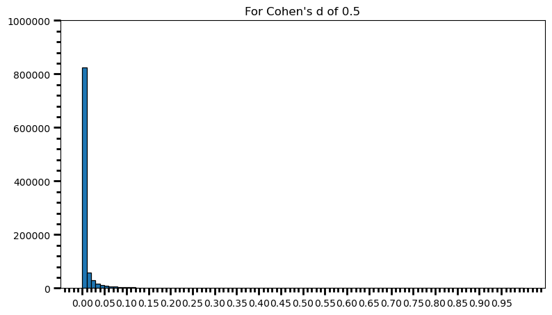
As one can see, statistical power also depends on the sample size and it should make sense: p-value is a function of test statistic (t, in this case) and following from there, function of sample size. If this doesn’t feel comfortable to you, I suggest you to take a look at this post, and check what happens to standard error as the sample size increases.
In the examples below, we always knew the underlying distributions of the populations we sample from. In reality, we usually end up with a result and we wonder the true effect: What is the chance that there is an effect, given that I observed one. This conditional probability is called positive predictive value, something that I heard from a political scientist during pre-COVID days, and if you’re interested in these stuff I suggest you to take a look at it. You can start from Ioannidis’ paper or Lakens’ book for more structured follow.